Bayesian Estimation of G Train Wait Times
In the hope of not letting decent data go to waste, even if it's only 19 rows, this post is about pulling useful information from a weird, tiny dataset that I collected during the summer of 2014: inter-arrival times of the G train, New York City's least respected and (possibly) most misunderstood subway line.
The only non-shuttle service to not touch Manhattan, the G is known to suffer from relatively threadbare scheduled service. It even has fewer cars than other lines and as a result is much shorter, like it's yet to reach puberty. I've been totally reliant on it for years however, as have many other people who live in Brooklyn, and am very interested in the extent to which it actually does operate relative to its reported badness. This led me in part to spend a few weeks imputing G train inter-arrival times (i.e. the times between trains) onto my iPhone every morning during my commute. I am potentially the only person to have ever done this for free, but I am glad I did because now I can use this data to build a simple model to estimate wait times between G trains.
This data also presents an opportunity to highlight a cool Bayesian conjugate prior relationship that I have seen fleshed out only once or twice, which is that between the exponential and gamma distributions. In explaining the framework of Bayesian updating rules (and the Bayesian philosophy generally), wherein we update our beliefs about outcomes with data on the likelihood of these outcomes, the relationship between the beta and binomial distributions is often used as an introductory example. This may take the form, for instance, of updating our prior beliefs about whether a coin is fair or unfair (the beta distribution) with actual flips of that coin (the binomial distribution). As a learning example, this is useful but a bit odd — what is an "unfair coin" and what would one look like if such a thing existed? (here is an actual report (pdf) written by noted statisticians on this subject). A similarly straightforward but potentially more useful procedure can be performed if one has an exponentially distributed random variable (in our G train example, of wait times) and prior information about this variable.
This is basically meant to be an introductory sort of post, but if you're a dyed in the wool Bayesian you'll hopefully appreciate the brevity of the expository parts.
Expecting to wait
Say we're interested in estimating the time we'll have to wait for the arrival of a G train, so we start to collect data on the times between trains. We obtain the first and second day's measurements, and it's not what we expect. For both days there's a fairly short time between trains — only 3 and 4 minutes.
Would you expect this to be an accurate representation of the average time between trains? No, probably not. These are obviously just two data points, and a three minute wait time does not exactly measure up to data on the G train's scheduled service from the MTA. We should of course collect more data, but in these early stages when we have so little of it, is it fair to totally discard the legitimate (as in, empirically backed) belief that the average time between G trains is longer than 3 or 4 minutes?
In statistical parlance, these expectations about how long we're going to wait for the train are called "prior expectations" — they are expectations about what will happen that are (usually) independent of the data we actually collect. The vast majority of statistical analysis treats prior expectations about experimental outcomes, if you have them, as totally separate from the data you collect; the data is all that matters, even if you're only able to turn up 19 rows of it. This approach has dominated 20th century experimental statistics and is referred to as frequentist statistics, and the method of incorporating prior expectations about outcomes is known as Bayesian statistics, after the 18th century English statistician who derived the framework's most important algorithm, Bayes theorem.
At the risk of discarding the nuances of a century long debate in the natural and social sciences, for the purposes of this post it's better to hold off judgement as to the relative merits of these methodologies. Suffice it to say that it would clearly be beneficial to incorporate our prior expectations of G train wait times into this problem, especially with a very small dataset, and that Bayesian estimation provides an elegant way to do so. As we collect more and more data, this methodology will also ensure that these prior expectations are eventually overwhelmed by the data we collect as we collect a sufficient amount of it. It also doesn't hurt that our formulation of the problem can be made simple enough that we can utilize only simple mathematical rules — the aforementioned conjugate relationship between the exponential and gamma distributions — rather than more involved computer simulations (as is usually the case with Bayesian analysis) to incorporate our prior expectations with our data.
The data
Let's take a look at the data in R. The full dataset can be found here.
head(gtrain)

#         date time1 time2 diff
# 1 2014-06-17   814   817    3
# 2 2014-06-18   853   857    4
# 3 2014-06-24   803   820   17
# 4 2014-06-25   807   817   10
# 5 2014-06-26   805   816   11
# 6 2014-06-27   813   817    4
I recorded two train arrivals per day, and the time between trains is in the fourth column. If we're interested in determining the probability of waiting a certain amount of time for a train's arrival, then we need to fit this time difference data to a probability distribution. The single parameter exponential distribution is often used to model wait times, and it is easy enough to estimate its parameter using the method of moments, wherein the exponential's "rate" parameter is equal to the inverse of the mean of the data.1 1 One important, simplifying assumption we have to make in this model is that the arrival of every G train occurs independently from the trains that come before or after it. Independent events that occur at a constant known rate are examples of what are called "Poisson processes". By making this assumption for the G train, we're estimating arrival times in a sort of idealized scenario in which a train's delay due to maintenance issues doesn't effect the trains that proceed it. Taking the first two measurements, we'd have an average wait time of 3.5 minutes. A bad wait time for me is at least 10 minutes, but with this mean there'd only be a 6% chance of this happening. Here's what the exponential distribution looks like plotted with this parameter.
library(ggplot2)
theme_set(theme_classic())

exp.rate <- 1 / mean(gtrain$diff[1:2])

exp.x <- seq(0, 30, length  = 100)
exp.y <- dexp(exp.x, rate = exp.rate)

ggplot(data.frame(exp.x, exp.y), aes(exp.x, exp.y)) +
  geom_line(color = "#0BD318") +
  geom_vline(xintercept = 10, linetype = "longdash") +
  xlab("minutes between trains")

1 - pexp(10, exp.rate)

# 0.05743262

Here, the area under the curve to the left of the line is the probability that we'll wait less than 10 minutes, and to the right that we'll wait more than this amount of time. For the G, we'd expect more area under these longer times. We don't really have that here, so let's restart and begin again as Bayesians by estimating a prior for our data.
How long we expect to wait
We'd hope to have more than anecdotal evidence to support our beliefs about the G, and thankfully it comes from the MTA. Taking a look at the schedule for the train (pdf), the Nassau stop (where I collected my data) sees a train "every 7 - 9" minutes between 8 AM and 9 AM. Compared with other trains, this is a long time to wait. Let's say that over the course of an hour, we see 8 trains, meaning our average wait time is 7.5 minutes.
One of the key points of Bayesian estimation is to not only incorporate our prior beliefs regarding event outcomes, but to preserve the uncertainty we have regarding them. In this context, this means that we expect that there are 7.5 minutes between trains, but possibly longer and possibly shorter, with some degree of certainty either way. As we're actually estimating a parameter for the exponential distribution, we need to estimate the probability that this parameter may take on any positive value.
The gamma distribution is our choice of distribution to fit this parameter, as it is a conjugate prior to the exponential. Here is a table of distributions that have conjugate priors, details about their parameters, and how they're related mathematically. Most of these can only be used in very simple cases, but ours in one such simple case.
The mean that we expect is 7.5 minutes, and since we need to fit the exponential distribution's parameter, we need the inverse of this mean. The gamma has two parameters, called a shape and rate parameter. In the context of a prior, the shape parameter is equal to the number of observations of our waiting time event, and the rate is the sum of these observations (or, just our total waiting time). Let's take a look at what this gamma distribution will actually look like.
gamma.prior.shape <- 8
gamma.prior.rate <- 60

gamma.x <- seq(0, .4, length  = 100)
gamma.prior.y <- dgamma(gamma.x, shape = gamma.prior.shape, rate = gamma.prior.rate)

ggplot(data.frame(gamma.x, gamma.prior.y), aes(gamma.x, gamma.prior.y)) +
  geom_line(color = "#0BD318") +
  xlab("exponential parameter value")
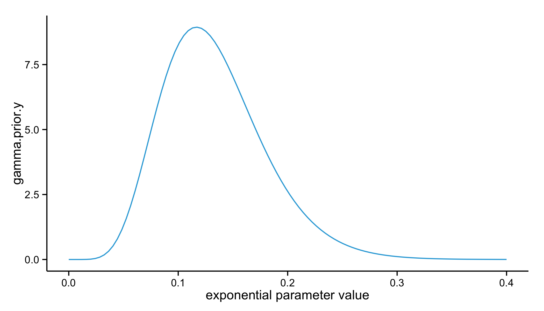
If we were to take a random sample from this distribution, it could take on a range of parameter values, but our best guess is the mean of the distribution (given its shape, the median would also be appropriate). What would this parameter look like once it's plugged into the exponential distribution?
exp.prior.rate <- gamma.prior.shape / gamma.prior.rate
exp.prior.y <- dexp(exp.x, rate = exp.prior.rate)

ggplot(data.frame(exp.x, exp.y, exp.prior.y), aes(x = exp.x)) +
  geom_line(aes(y = exp.y, colour = "exp w/out prior")) +
  geom_line(aes(y = exp.prior.y, colour = "exp prior")) +
  geom_vline(xintercept = 10, linetype = "longdash") +
  scale_colour_manual(values = c("#0BD318", "#34AADC")) +
  labs(x = "minutes between trains", y = "y") +
  theme(legend.title=element_blank())

1 - pexp(10, exp.prior.rate)

# 0.2635971
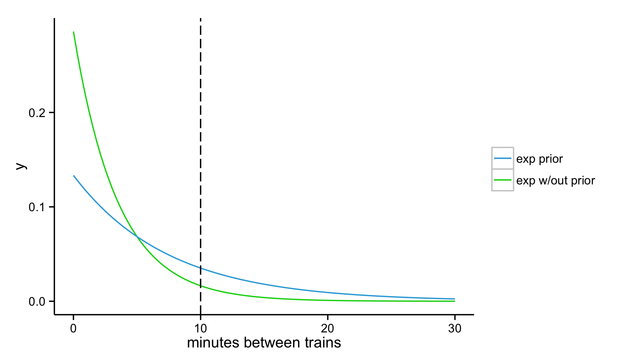
The MTA tells us that there's a 26% chance we'd wait longer than 10 minutes given the choice of these parameters, which is more in line with what we'd expect. Thanks to the conjugate relationship between the exponential and gamma distributions, we'll be able to combine both the estimate from our data — with only two data points, and then with all of the data we collected — and our estimate from the MTA.
Incorporating Prior Beliefs
Here's the part where we explore one of the joys of conjugate priors, which is the simplicity of updating our prior beliefs with actual data. Without going into the math of why this works (pdf), all we need to do to update our prior beliefs is to add the number of new observations to the gamma prior's shape parameter, and the sum of these new observations to its rate parameter. In doing so we shift the estimate of the most likely parameter for our exponential distribution, and thus of our expected wait time.
With our first two data points, we observed two additional trains with wait times that sum to a total of seven minutes. Here is our updated gamma distribution that incorporates this data relative to our original gamma distribution for our prior.
gamma.posterior.shape <- gamma.prior.shape + 2
gamma.posterior.rate <- gamma.prior.rate + sum(gtrain$diff[1:2])

gamma.posterior.y <- dgamma(gamma.x, shape = gamma.posterior.shape, rate = gamma.posterior.rate)

ggplot(data.frame(gamma.x, gamma.prior.y, gamma.posterior.y), aes(x = gamma.x)) +
  geom_line(aes(y = gamma.prior.y, colour = "gamma prior")) +
  geom_line(aes(y = gamma.posterior.y, colour = "gamma posterior")) +
  scale_colour_manual(values = c("#0BD318", "#34AADC")) +
  labs(x = "exponential parameter value", y = "y") +
  theme(legend.title=element_blank())
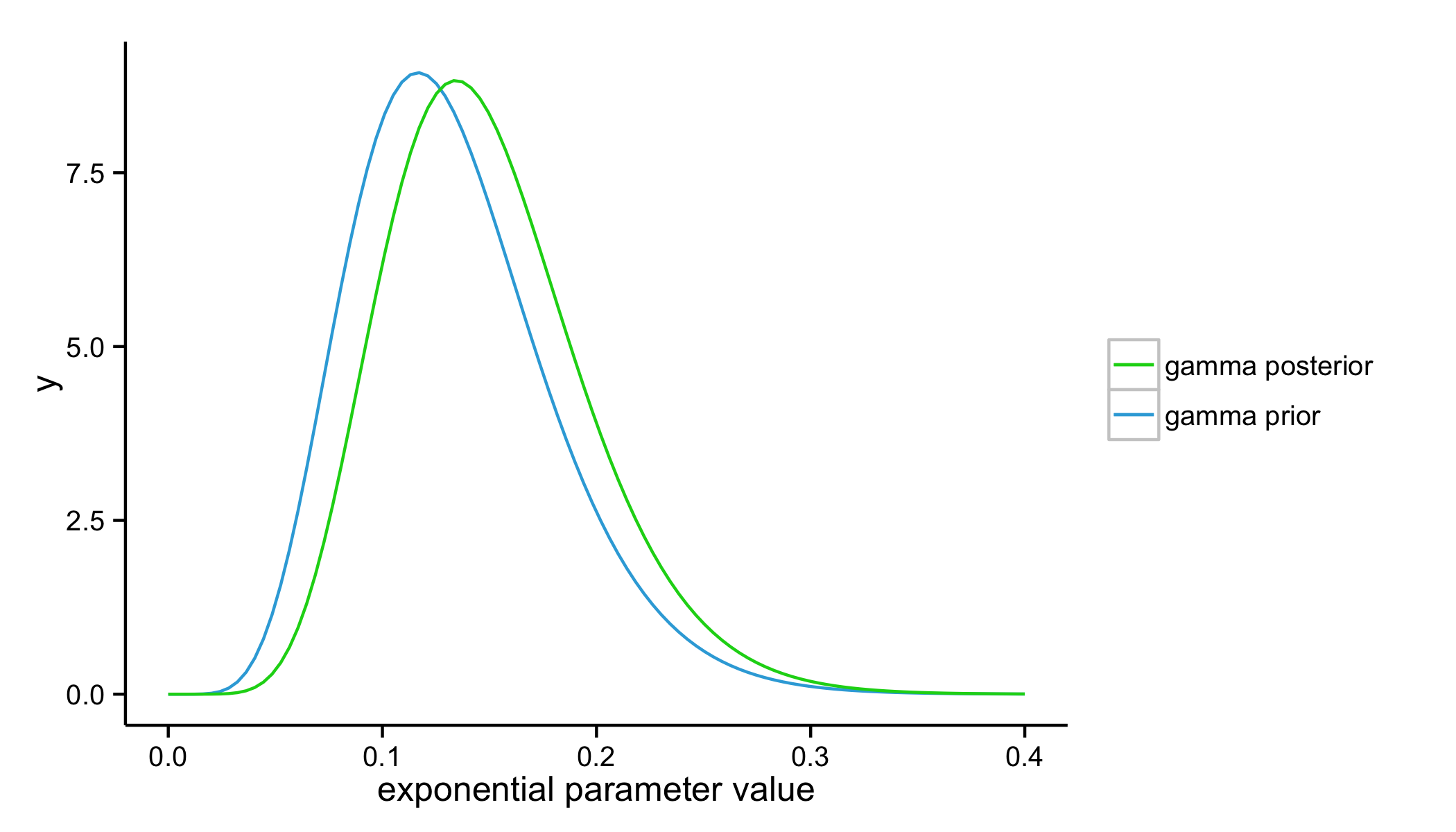
Notice how the distribution has shifted to the right a bit. Its mean will have also shifted to take on larger values. For the exponential distribution, this means a smaller rate parameter and a smaller estimated waiting time.
exp.posterior.rate <- gamma.posterior.shape / gamma.posterior.rate
1 - pexp(10, exp.posterior.rate)

# 0.2248015
By combining our prior belief that there's a 26% chance of waiting more than 10 minutes for a G train with our first two observations that there's only a 6% chance, we've ended up somewhere in the middle. That "somewhere" is weighted more heavily towards our prior, which makes sense — after all, we've only observed two wait times. The great thing about this procedure is that as we collect more data we can repeatedly update our estimation and arrive at a more precise, empirically backed estimate. Now let's throw the rest of our dataset at this problem and see what we get.
exp.full.posterior.rate <- (gamma.posterior.shape + (nrow(gtrain) - 2)) / (gamma.posterior.rate + sum(gtrain$diff[3:length(gtrain$diff)]))
exp.full.posterior.y <- dexp(exp.x, rate = exp.full.posterior.rate)

ggplot(data.frame(exp.x, exp.prior.y, exp.full.posterior.y), aes(x = exp.x)) +
  geom_line(aes(y = exp.prior.y, colour = "exp prior")) +
  geom_line(aes(y = exp.full.posterior.y, colour = "exp full posterior")) +
  geom_vline(xintercept = 10, linetype = "longdash") +
  scale_colour_manual(values = c("#0BD318", "#34AADC")) +
  labs(x = "minutes between trains", y = "y") +
  theme(legend.title=element_blank())

1 - pexp(10, exp.full.posterior.rate)

# 0.1966153
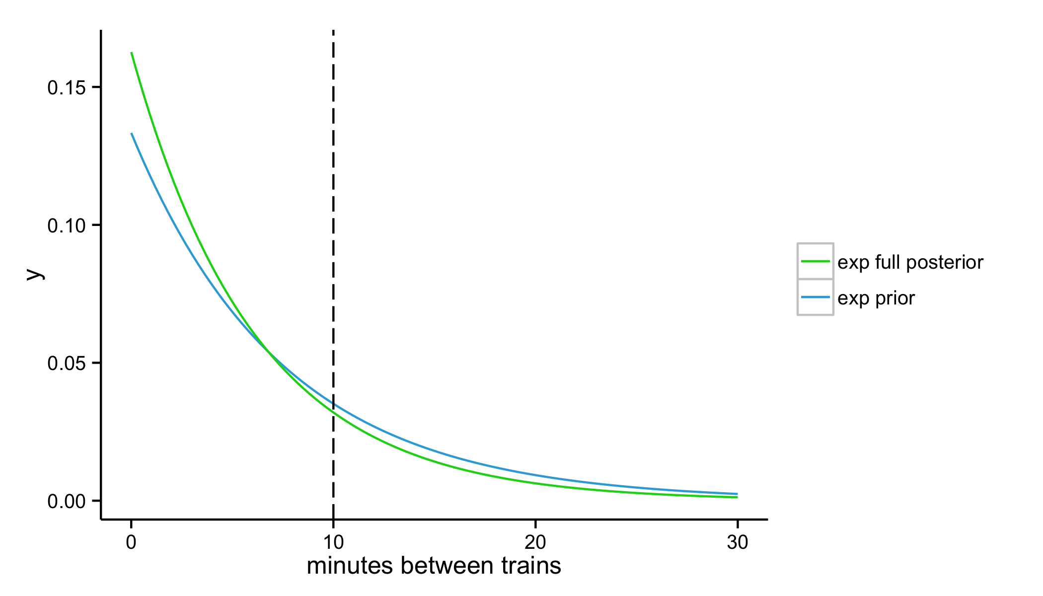
By incorporating all of the data I collected over 19 days, we've arrived at a sunnier 20% chance of waiting more than 10 minutes for a G train to arrive. The difference between our prior and our full posterior estimation is not huge, but if we were to continue to see the fairly modest wait times I experienced over those 19 days it seems like we'd actually end up redeeming the G train's name to some extent (at least during morning commuting hours).
This is a simple problem and we've made several assumptions, but I think it makes clear the utility and appeal of Bayesian estimation methods. In allowing for the probabilistic estimation of event outcomes and the updating of these probabilities with evidence, it also seemingly comports with how we naturally make everyday decisions.
Feel free to reach out about anything and everything!